Understanding Spatial Join in Unfolded Studio

A fundamental operation in GIS and spatial data science, spatial join combines two datasets based on their spatial relationships to address spatial analytical pain points and derive business insights. Unfolded’s browser-based spatial join function is fast and intuitive and can be performed on 9 million points with 157 polygons in 8 seconds – the fastest we have ever seen compared to existing platforms.

What is Spatial Join

To start, let’s break down what spatial join is exactly. Nowadays, millions of geo-location data are generated every second, such as geo-tagged photos and videos, lidar geo-point cloud, real-time location of delivery trucks, electric rental scooters, ride-share vehicles and even the food you just ordered online. However, analyzing these geospatial data and deriving valuable insights becomes a challenge for data scientists, researchers, and decision-makers.

In the Unfolded Studio, we provide several tools to analyze the raw geolocation data. For example, we can use the Cluster layer to visualize aggregated data based on a geospatial radius, use the Heatmap layer to visualize the intensity of data at geographical points through a colored overlap, or use the Flow layer to visualize origin-destination movement patterns.

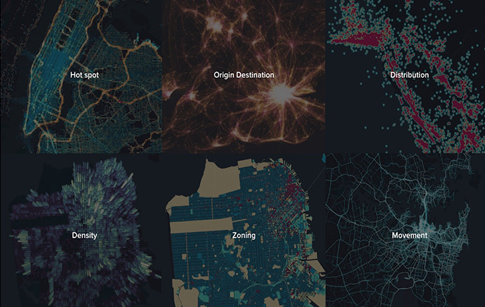
Unfolded Studio analytical tools

In real-world applications, one of the most commonly-used data processing steps is to join the raw spatial data with other spatial analytical units (e.g. administrative boundaries, custom-defined regions or road networks) so that data analysis can be applied on a proper spatial scale and the conclusions (e.g. patterns and knowledge) can be drawn on a meaningful spatial unit. This join operation combining different geospatial datasets based on geolocation is what’s known as spatial join.

Using Spatial Join in Analysis

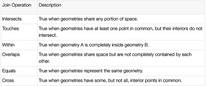
Technically, spatial join is a query operation that identifies all pairs of spatial objects that satisfy a predefined spatial relationship, such as intersection, within and touch, in order to aggregate the values based on the query results. Unfolded Studio supports six spatial join query operations:

Since spatial join can tell you the spatial relationship between spatial entities, we can use it to answer many spatial analytical questions, such as:

• Which houses are within the high flood risk zones
• Which street in the city has the most car accidents
• Which community has the most parking violations
• Which part of the city has the most/least electric scooter rentals
• What is the total house footprint area within the zip code area

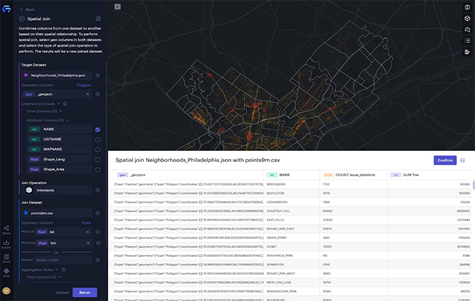
Let’s say you have a dataset of millions of parking tickets within a city. Each parking ticket has a geolocation representing where it has been issued. Your goal is to analyze how many tickets are issued and the total amount of fines for each neighborhood in the city.

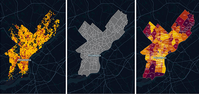
Spatial joining the events (points) to the neighborhoods (polygons)

For example, you can run a spatial join on parking tickets (the points indicated in the figure above) with the neighborhood boundaries (the polygons) in order to understand which points are within which neighborhood area; from there, you are able to compute the total amount of fines by aggregating the fine amount of each ticket. The number of tickets and the total amount of fines can be attached to each neighborhood as the final result.

However, spatial joins are not just limited to points inside polygons. Unfolded Studio supports 52 combinations of different features (points/polygons/lines) and join operations:

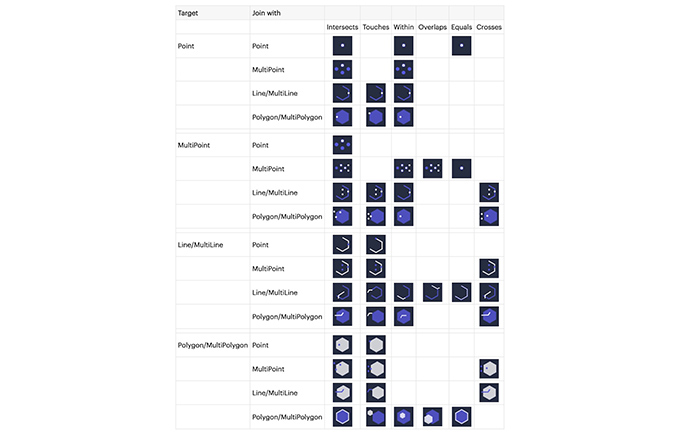
Unfolded Studio’s various features and join operation combinations

In Unfolded Studio, each of the above spatial join types can be executed for millions of data points in seconds, and all within your browser. This means you don’t need to write any code or SQL query – all you need is a free community account to get started.

Performing Spatial Join in Unfolded Studio

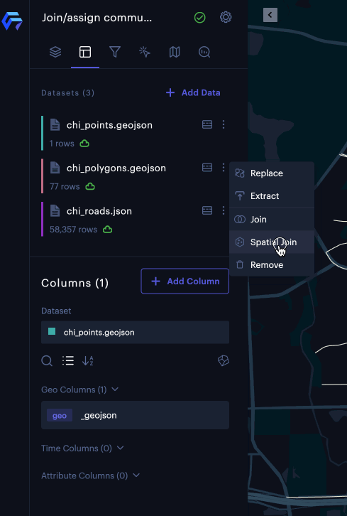
To perform spatial join in the Unfolded Studio, you can click the icon ⋮ on any dataset with a geometry column and click “Spatial Join” in the popup menu. (see the left figure below). Once you select spatial join, a side panel appears with configuration options for the spatial join feature. (see the right figure below).

The Spatial Join menu option (left) and Spatial Join panel (right).

The Spatial Join panel contains three sections:

• Target Dataset: Configures the dataset you will join against
• Join Operation: Selects a supported join operation between the source and target dataset.
• Join Dataset: Selects columns and specifies aggregation rules (how to aggregate results when joining multiple rows). The supported aggregation rules include: Count, Sum, Mean, Max, Min, Deviation, Variance, Median, Percentile (P05, P25, P50, P75, P90)

You can specify geometry columns for both datasets and select the type of spatial join you want to perform. From there, you can click the “Run” button to run spatial join. Once the operation is complete, you will review the new joined dataset with joined results in a data preview panel and select “Confirm” once everything is set. Voila, a new map layer will be created based on the joined dataset.

Based on the geometry types you selected in both datasets, Unfolded Studio suggests an appropriate join type.

Performance Comparison

We implemented the optimized spatial join in C++, which was then compiled into a WebAssembly module that runs in the browser. To get even better performance, we also introduced web workers to parallelize the spatial join.

In order to compare the performance, we use the ~9 million-record set of parking infractions data from Philadelphia and join it to a 157-record set of Philadelphia neighborhoods. This data has been used in other spatial join performance tests, with Crunchy Data reporting that the join execution of the parking infractions with the neighborhoods took about 24 seconds using a dedicated Postgresql server with 32GB memory and 8 virtual CPU cores. However, this report also shows an extra 60 seconds for creating the spatial index.

The results of spatial join ~9 million record of parking tickets with 157 neighborhoods

We then transferred the same spatial join tests using the Google Big Query. After spending some time loading the datasets, we ran spatial join using SQL query in the Big Query web interface directly. This took about 18 seconds to run, but it’s worth noting that the input stage in the query took about 18 seconds and the join stage only took about 3 seconds. Here lies one of the key advantages: the spatial index has been prebuilt to improve the performance while loading the datasets into the Big Query and the Unfolded Studio provides a connector to Google Big Query.

It doesn’t stop there. We have also run these same spatial join tests using GeoPandas ( 0.10.2) and pyGEOS ( 0.10.2) on a 2020 MacBook Pro with an M1 chip (8 cores and 16GB memory). We used geopandas.tools.sjoin with the spatial index for spatial join operation in Python 3.8 (x86_64). It took about 2 seconds to create the spatial index and 26.8 seconds to run the spatial join task, so 28.8 seconds in total.

Using Unfolded Studio on the same machine, the task took only about 8 seconds with 6 web workers in the Chrome browser. It’s much faster than the tests using the Postgresql server and GeoPandas+pyGEOS. Besides the performance comparison, the best part of using Unfolded Studio is that you can do “point-and-click” spatial join in the browser without the need to write any code or create a database to run SQL queries.

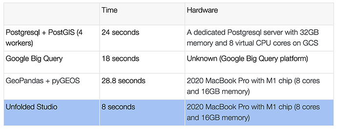
Performance comparison when joining 9 million points with 157 polygons

Spatial Join IRL

Example 1. Aggregating millions of parking infractions data for 157 neighborhoods in Philadelphia.

The parking infractions data include millions of points and each one represents the location of a parking violation ticket. Using spatial join, we can aggregate the points to each neighborhood based on the geographic locations. In this example, we demonstrate how to compute the total amount of fines for parking violations in all neighborhoods across Philadelphia:

1. Select the Spatial Join option from the dataset “Neighborhoods_Philadelphia.json.”
2. In the Spatial Join panel, we select the Join Dataset: “Parking Violations.csv”. Unfolded Studio will automatically detect the geometry type “Point” and geometry column: “lat” and “lon.”
3. Make sure the Join Operation selection is Intersects, which means all the points within or touch the polygon are considered as valid spatial join.
4. Click on the field selector of fine column under the Attribute Columns(1) label, and choose Sum as the aggregation rule in the pop-up menu. By doing so, we can compute the sum of the fine value of all points joined with each neighborhood.

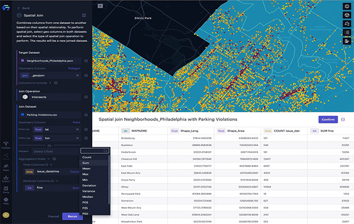
Spatial joining the parking infractions data with 157 neighborhoods in Philadelphia.

The result of the spatial join is a new dataset with a column “COUNT issue_date,” which represents how many data points (tickets) are in each polygon (neighborhood), and a column “SUM fine,” which represents the total amount of fines from all data points in each neighborhood. We can then create a thematic map using the new column “SUM fine” to show the spatial distribution of the infractions data at the neighborhood level.

Example 2. Spatial joining 177,023 building footprints with 25 zip code areas in San Francisco.

We are now going to use spatial join on 25 zip code areas with 177,023 building footprints in San Francisco, in order to compute 1) how many buildings and 2) what the total area of these buildings in each zip code area are.

1. Select the Spatial Join option from the dataset “sfzip.json.”
2. In the Spatial Join panel, we select the Join Dataset: “sf.buildings.json.” Unfolded Studio will automatically detect the geometry type “Polygon” and geometry column: “_geojson.”
3. Make sure the Join Operation is Intersects, which means all the polygons (buildings) intersect with the zip code area are considered as valid spatial join.
4. Click on the field selector of mblr (San Francisco property key) column under the Attribute Columns(2) label, and choose Count as the aggregation rule in the pop-up menu. By doing so, we can count how many building footprints intersect with each zip code area.
5. Click on the field selector of area (The area of building in square meters) column under the Attribute Columns(2) label, and choose Sum as the aggregation rule in the pop-up menu. By doing so, we can compute the total area of the building footprints intersecting with each zip code area.

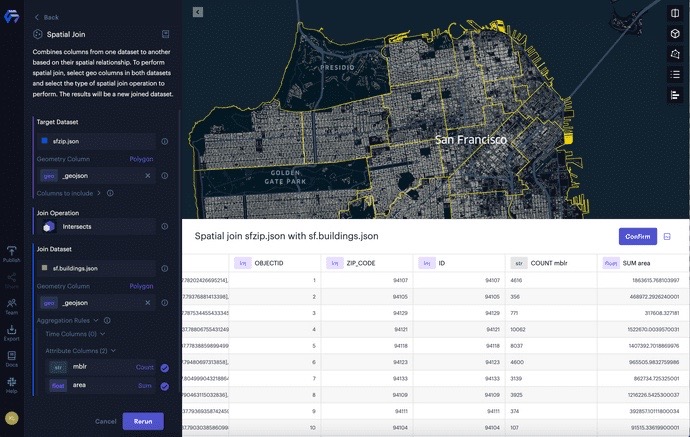
Spatial joining the building footprints with zip code area in San Francisco.

The result of the spatial join is a new dataset with a column “COUNT mlbr,” which represents how many building footprints in each zip code area, and a column “SUM area,” which represents the total area of the building footprints in each zip code area. From there, we can create a thematic map using the new column “SUM area” to show the spatial distribution of the total area of building footprints at the zip code level.

Interested in learning more? Register for our upcoming webinar on June 28th, where we’ll dive into Spatial Join and what’s to come for Unfolded.

You can also contact us for a demo of Unfolded to get started today!